Today's Excel tip for those less experienced users is how to use the FORECAST and TREND functions.
These functions can be extremely helpful if you sales data or any other series where there is a trend emerging and you want to predict future values.
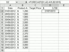
The examples below use the following sales data for Product A.
Looking at the data below we can see there is a clear upward trend in the sale price for Product A. The data we have used could be replaced for any product or service where has a clear trend emerging in the data.
For business owners this can be a handy tool to forecast sales targets or milestones for production.
Based on the data below, when is the price of Product A forecast to hit $3,700?
Jan-12 $1,250
Feb-12 $1,500
Mar-12 $1,800
Apr-12 $1,875
May-12 $2,000
Jun-12 $2,200
Jul-12 $2,240
Aug-12 $2,400
Sep-12 $2,370
Oct-12 $2,400
Nov-12 $2,500
Dec-12 $2,600
Jan-13 $3,000
Feb-13 $3,200
If we set the data up in Excel with the dates in Column A, the sales values in Column B, and the target price in cell C1, then in cell C2 we would type the following formula =FORECAST(C1,A1:A15,B1:B15)
In cell C2 the result returned in excel should be 21 July 2013. If however you get a number like 41,476.18, don't panic, this is how Excel returns dates when the cell is not formatted to show the date.
To resolve this simply click on the cell with the number in it (i.e. C2) and press CTRL + 1, this will bring up the Format Cells command box and you then choose Date from the list and select the appropriate format for the date (e.g. dd/mm/yyyy).
Alternatively you can also find the same command box by going to the tool bar and selecting Format then Cells from the drop down menu. For those who like using shortcuts using the key board while holding down the ALT key press the 'O' key followed by the 'E' key.
Another forecasting tool we can use is via the TREND function in Excel.
Using the same data as before if we insert the dates Mar-13, Apr-13, May-13, Jun-13 and Jul-13 into cells A16:A20 and in cell B16 type the formula =TREND($B$2:$B$15,$A$2:$A$15,A16,TRUE) we can forecast what the price of Product A could be in March 2013 based on the trend of the previous data. The resulting price in cell B16 is $3,158.
Copying the formula down we get the following values $3,279, $3,404 $3,525 and $3,650. The last value is the "forecast" price of Product A at the end of July 2013 based on the previous trend.
We can see that while the price is forecast to hit $3,700 on 21 July 2013 at the end of the month based on the TREND formula the price is expected to be $3,650 which is pretty close.
If you do not enter the $ sign (absolute cell reference) as noted in the formula you will come out with different results as for each new entry down the page the cell ranges in the formula move down one position and drops off one of the previous observations.
Why do these two methods produce slightly different results?
The FORECAST function in Excel calculates, or predicts, a future value by using existing values. The new value is predicted by using linear regression.
On the other hand, the TREND function returns values along a linear trend and the data fits a straight line (using the method of least squares) based on the known and unknown values. The TREND calculation is in effect smoothing the data to fit a line
There are subtle differences in the way these two calculations operate. Predicting future values will never be a perfect process and variability in outcomes should be expected. .
A final note on the syntax in the formula
The words TRUE or FALSE in the formula are optional.
For those with an understanding of statistics and regression if the last argument "constant" is set to TRUE, you want the regression model to include a coefficient for the intercept in the regression model. If the last argument is set to FALSE, no intercept term is included; the fitted regression is forced to go through the origin. The last argument is optional; if omitted it is interpreted as TRUE.
---------------------------------------------------------------------------------------------
We encourage you to use the comment section below to add in your own tips about this function. Or ask a question ...
We welcome your comments below. If you are not already registered, please register to comment
Remember we welcome robust, respectful and insightful debate. We don't welcome abusive or defamatory comments and will de-register those repeatedly making such comments. Our current comment policy is here.